Normalization and denormalization can be approached in two contexts. The first context has to do with the deduplication of data and query speed on database tables in a relational database. The other context has to do with the normalization of data values in a machine learning scenario. Starting with the first context, begin with a review of the following descriptions of different database normal form rules which are used to normalize data. There are many normalization rules, but the most common are 0NF, 1NF, 2NF, and 3NF. 0NF does not qualify as one since it is considered to have no normalization.

Database Tables

0NF
This level of normal form is not considered normalized at all. It is not efficient for querying or searching, and the structure is not flexible.

Notice that some columns have similar, repeating names. Having attributes that repeat, like ELECTRODE1, ELECTRODE2, etc., is poor design in that it lacks flexibility.

1NF
The objective for the first normal form is to remove any repeating groups, such as the columns ELECTRODE1, ELECTRODE2, ELECTRODE3, etc. The data in this normal form is two dimensional because a MODE has multiple ELECTRODEs. The repeating columns can be replaced with a new ELECTRODE table, as follows:

You might be able to visualize why 1NF is easier to search when compared to 0NF. Think about a piece of information you would want to retrieve from the BRAINWAVE table. For example, which SCENARIOs are related to ELECTRODE_ID = 5? In 1NF you can use the ELECTRODE table and a JOIN to find the sought after piece of information. In 0NF, you would need to write a query that checks each column, to determine which column contains Pz. That is not very efficient. From a flexibility perspective, what happens if you want to add a new electrode? If the table is in 0NF, it requires a new column, but 1NF requires only an additional row of data in the ELECTRODE table.

2NF
The objective of the second normal form is to remove redundant data and to ensure that the BRAINWAVE table contains an entity with a primary key comprising only one attribute. In this example the duplicated data is removed from the BRAINWAVE table by adding the ModeElectrode table with a key of MODE_ID + ELECTRODE_ID. ELECTRODE_ID is removed from the BRAINWAVE table and placed into the ModeElectrode table, which contains the relationship between MODE and ELECTRODE. An entity is in 2NF if it has achieved 1NF and the additional requirements. The following tables represent the 2NF requirements. Notice that the duplication is removed.

The ModeElectrode table identifies and maintains the relationship between MODE and ELECTRODE. This results in the deduplication of data in the BRAINWAVE table.
ModeElectrode

The ELECTRODE table remains the same in this scenario, as it is required to comply with and achieve 1NF.

The ELECTRODE table is useful in JOINs, which will provide the name of the ELECTRODE and its link to the MODE.

3NF
An entity or table is in 3NF if it is 2NF and all its attributes are not totally dependent on the primary key in the BRAINWAVE table. For example, the SESSION_DATETIME in the SESSION table is transitively dependent on SCENARIO.

A new SCENARIO table must be created in order to enable the removal of the SESSION_DATETIME column attribute from the BRAINWAVE table.

In order for both the ModeElectrode and ELECTRODE tables to achieve 3NF, they must comply with 2NF requirements also. To be considered 3NF, the entity must also be 2NF‐compliant.
ModeElectrode

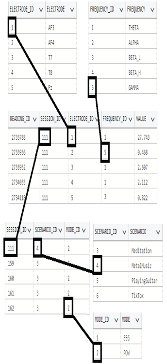
The reverse of what you just read concerning normalization rules is what you would call denormalization. The reason you would denormalize data is to reduce the number of JOINs required to retrieve a desired dataset. A JOIN is a high‐impact command. Running a SQL statement that contains many JOINs on large datasets will likely be more latent when compared to queries with fewer JOINs. Consider some of the previous exercises in this chapter in which you transformed data. An aspect of that was the denormalization of the data. An example is with the data that was pulled from a relational Azure SQL database with the structure illustrated in Figure 5.28, which is 3NF. The transformation employed JOINs over numerous reference tables. The resulting dataset was a single compact table that contained all the information necessary for exploratory analysis that requires no JOINs. The boxes show the connections between the tables.
The next bit of content enters the realm of machine learning, which is not something you would likely encounter on the DP‐203 exam. However, as you progress into exploratory data analysis, the normalization of data values can help you visualize data in a more consumable manner.

FIGURE 5.28 Normalizing and denormalizing brainjammer values