- Log in to the Azure portal at https://portal.azure.com ➢ navigate to the Azure Synapse Analytics workspace you created in Exercise 3.3 ➢ on the Overview blade, click the Open link in the Open Synapse Studio tile ➢ navigate to the Develop hub ➢ create a new notebook ➢ select PySpark (Python) from the Language drop‐down list box ➢ open the file normalizeData.txt on GitHub at https://github.com/benperk/ADE in the Chapter05/Ch05Ex10 directory ➢ and then copy the contents into the notebook.
Notice that the input for normalization is the same as the data shown in the previous data table.
- Select your Spark pool from the Attach To drop‐down list box ➢ click the Run Cell button ➢ wait for the session to start ➢ and then review the results, which should resemble the following:
- Consider renaming your notebook (for example, Ch05Ex10), and then click Commit to save the notebook to your source code repository.
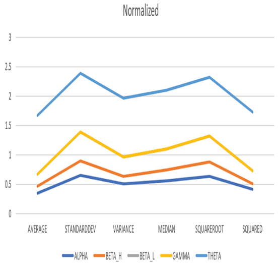
The aspect of the resulting normalized data you may notice first is the existence of the 1.0 and 0.0 values. This is part of the normalization process, where the highest value in the data to be normalized is set to 1.0, and the lowest is set to 0.0. It just happened in this case that the GAMMA readings were all the smallest and THETA were the largest in each reading value calculation. Using the normalized data as input for a chart renders Figure 5.30, which is a bit more pleasing, interpretable, and digestible.
The classes and methods necessary to perform this normalization come from the pyspark.ml.feature namespace, which is part of the Apache Spark MLlib machine learning library. The first portion of the PySpark code that performs the normalization manually loads data into a DataFrame.

FIGURE 5.30 Normalized brain waves data
The next line of code defines a loop, which will iterate through the provided columns to be normalized.
for b in [“AVERAGE”, “STANDARDDEV”, “VARIANCE”, “MEDIAN”, “SQUAREROOT”, “SQUARED”]:
The VectorAssembler transformation class merges multiple columns into a vector column. The code instantiates an instance of the class by passing the input data columns to the class’s constructor. The result of the merge is stored into the outputCol variable, which includes column names appended with _Vect. A reference to the class instance and the result are loaded into a variable named assembler, which is a Transformer abstract class. The transformer is often referred to as the model, which is a common machine learning term.
assembler = VectorAssembler(inputCols=[b],outputCol=b+”_Vect”)
The MinMaxScaler class performs linear scaling, aka normalization, or rescaling within the range of 0 and 1, using an algorithm similar to the following:
z = x – min(x) / max(x) – min(x)
The line of code that prepares the data for min‐max normalization is presented here. The code first instantiates an instance of the class and passes the data columns to the constructor with an appended _Vect value. The result of the normalization will be stored into the outputCol variable with an appended _Scaled value on the end of its column name. A reference to the class instance and the result is loaded into a variable named scaler which is an Estimator abstract class.
scaler = MinMaxScaler(inputCol=b+”_Vect”, outputCol=b+”_Scaled”)
The pipeline in this scenario is the same as you have learned from the context of an Azure Synapse Analytics pipeline, in that it manages a set of activities from beginning to end. In this case, instead of calling the steps that progress through the pipeline “activities,” they are called “stages.” In this case, you want to merge the columns into a vector table and then normalize the data.
pipeline = Pipeline(stages=[assembler, scaler])
When the fit() method of the Pipeline class is invoked, the provided stages are executed in order. The fit() method puts the model into the input datasets, then the transform() method performs the scaling and normalization.
df = pipeline.fit(df).transform(df) \
.withColumn(b+”_Scaled”, unlist(b+”_Scaled”)).drop(b+”_Vect”)
The last step appends the DataFrame with new normalized values using the .withColumn(). Those normalized values can then be used for visualizing the result.
Denormalization
The inverse of normalization is denormalization. Denormalization is used in scenarios where you have an array of normalized data and you want to convert the data back to its original values. This is achieved by using the following code syntax, which can be run in a notebook in your Azure Synapse Analytics workspace. The code is available in the denormalizeData.txt file, in the Chapter05/Ch05Ex10 directory on GitHub. The first snippet performs the normalization of the AVERAGE column found in the previous data table.
array([0.35041577,0.1150843,0.20360279,0,1])
To convert the normalized values back to their original values you perform denormalization, which is an inverse of the normalization algorithm.
denormalized = (normalized * (data_max – data_min) + data_min)
denormalized
array([8.03769,4.15734,5.61691,2.25973,18.7486])
You might be about the usefulness of this, as you already know what the original values are. In this case there is no need to denormalize them. Denormalization is very beneficial in testing machine learning algorithms. Machine learning involves predicting an outcome based on a model that is fed data—normalized data. The ability to denormalize normalized data enables you to test or predict the accuracy of the model. This is done by denormalizing the outcome and comparing it to the original values. The closer the match, the better your prediction and model.
