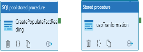
One action you may have noticed in Exercise 5.1 is that you used the existing pipeline that you created in Exercise 4.13. That pipeline performed one activity, which was to copy data from the Azure SQL database into the dimension tables and a temporary table that were created on a dedicated SQL pool in Azure Synapse Analytics. The temporary table tmpREADING had the same structure as the READING table on Azure SQL. The objective now is to get the data on the tmpREADING table to map into the FactREADING table. This was achieved by adding a SQL pool stored procedure to the pipeline that ran after a successful data copy. Note that there also exists a Stored Procedure activity in the General folder that is not the same as a SQL pool stored procedure. Figure 5.5 shows the difference.

FIGURE 5.5 Azure Synapse Analytics—SQL pool vs. a linked service stored procedure
The primary difference between the two is that the SQL pool stored procedure targets a dedicated SQL pool directly, whereas the other requires a linked service. Here is what the stored procedure code looks like:
CREATE PROCEDURE brainwaves.uspCreateAndPopulateFactReading
AS CREATE TABLE [brainwaves].[FactREADING]WITH
The stored procedure code creates a fact table with a hash distribution type on the frequency column. Remember that the values of frequencies can be THETA, ALPHA, BETA_L, BETA_H, and GAMMA. The CTAS SQL statement uses the dimension tables to convert the numeric representations of the scenario, electrode, and frequency into their actual friendly, easily identifiable names.
It is possible to learn from even the simple queries you ran in step 7 of the Exercise 5.1. The two queries that selected the count from the tmpREADING and FactREADING tables are useful to make sure the query that populated them includes the expected values. In this scenario you would expect the number of rows in each table to be the same.
The second query was unexpected and triggered some actions to determine why there were so many more brainjammer brain wave readings for the ClassicalMusic scenario versus the others. The data was skewed in the direction of that specific scenario, and the reason for this skew must be found. Recall from Figure 2.19 how a skew is generally illustrated.
The following SQL query resulted in the reason for the skew:
SELECT s.SCENARIO, COUNT(*) AS [COUNT]
FROM [brainwaves].[DimSESSION] se, [brainwaves].[DimSCENARIO] s
WHERE se.SCENARIO_ID = s.SCENARIO_ID
GROUP BY SCENARIOORDER BY [COUNT] DESC
It turns out the brainjammer brain wave data stored in the JSON files had not been completely parsed and loaded into the Azure SQL database. Missing sessions turn out to be the cause of the skew leaning heavily toward the ClassicalMusic scenario. You can see that there are 10 sessions for the ClassicalMusic scenario and only one for the others. In this case the data owner responsible for the data loading procedure was contacted, and the complete set of data was uploaded. Perform the same exercise using all the data available from all the sessions.
If you could not upload all the JSON files using the source code in file JSONToAzureSQL.cs, located in the Chapter02/Source Code directory, you can instead download the compressed database backup from the BrainwaveData/bacpac directory on GitHub at https://github.com/benperk/ADE.
You can download the ZIP file, extract the .bacpac file, and then import it into your own Azure SQL server. The credentials for the database backup are benperk for the server admin login and bra!njamm3r for the password. After importing the .bacpac file, consider rerunning Exercise 5.1.
